What Life Changes Can We Make Today To Avoid Obesity?
Project Goal
- Predicting obesity based on lifestyle habits
Introduction
This project was completed during my fifth week at Metis data science bootcamp. The learning objectives for this project were building a supervised learning (classification) model and deploying its product on a web app. I chose a topic that was dear to me, the obesity pandemic in the US.
According to the CDC, obesity-related diseases are the leading causes of death in the United States. People who are obese have higher chances of developing heart disease, hypertension, stroke, and even (some) cancers. With these statistics, I wondered: How much is the rise of obesity-related diseases influenced by our lifestyle? How does our (seemingly harmless) habit of snacking or dining out affect our chances of becoming obese? What is the impact of physical exercise, or its lack thereof, on our weight and overall health?
Data acquisition and pre-processing
To assess the health impacts of eating and exercise habits, I decided to build a classification model that is trained on a subset of American Time Use Survey (ATUS) Eating & Health Module Microdata Files, collected by the Bureau of Labor Statistics (also featured in Kaggle).
This dataset represents multi-year surveys that were conducted from 2006 to 2008 and from 2014 to 2016; It contains ~11,000 observations with 39 topics/questions related to weekly eating habits and other lifestyle choices. I chose body mass index (BMI) as the TARGET value to predict. According to CDC, people with BMI>30 are classified as obese, whereas others with BMI<30 are considered not obese. The ratio of obese and not obese was 72%:28%, an imbalanced class situation.
Splitting the dataset. I split the dataset into training (80%) and testing (20%) sets for model learning and evaluation, respectively. To reflect the ‘original’ imbalance scenario, I split the data using sklearn’s stratification feature. Then, I used random-oversampling (ROS) method from imblearn to obtain a balanced training set of obese and not obese classes, i.e., ~6,000 observations of each class.
Of the 39 survey questions, I decided to use five as my model FEATURES for my model for two reasons:
- From an end-user perspective, I wanted a simple app that requires the user to input only a few types of health data
- The five features were considered most important by Random Forest Classifier
Here are the five features:
- TimeEat, NUMERIC feature representing the original survey question of “What is the total time (minutes) spent eating and drinking (primary meals during the day)?”
- TimeSnack, NUMERIC feature representing the original survey question of “What is the total time (minutes) spent eating and drinking (primary meals during the day)?”
- ExerciseFrequency, NUMERIC feature representing the original survey question of_“During the past 7 days, how many times did you participate in any physical activities or exercises for fitness and health such as running, bicycling, working out in a gym, walking for exercise, or playing sports?”_
- FastFoodFrequency, NUMERIC feature representing the original survey question of “How many times in the last 7 days did you purchase: prepared food from a deli, carry-out, delivery food, or fast food?”
- GeneralHealth, CATEGORICAL feature representing the original survey question of_“In general, would you say that your physical health was excellent, very good, good, fair, or poor?”_
Building Classification Models and Their Classification Results
To consider models with high interpretability and predictive power, I examined Logistic Regression (LR) and Random Forest (RF) classifiers, respectively. I setup a pipeline that ran feature scaling and 10-fold cross-validation (CV) on each of the two classifiers. Grid-searching was also performed to find the best hyper-parameters. Finally, model performance was asessed using the (unseen) test set.
For the purpose of app deployment, the entire dataset was used for training. The trained model was embedded in a Python Flask app, which utilizes d3.js sliders as input method.
Checkout this web app, here.
Performance Evaluation. In general, the performance of Logistic Regression (LR) is comparable with that of Random Forest (RF) classfier (Figure 1). The LR model has a slightly higher accuracy than RF. However, the recall score for RF is better than that of LR. The latter is of great importance in healthcare, as it would be costly to misclassify someone who has an obesity-related disease as healthy. For this reason, I chose Random Forest as the classifier used in app deployment.
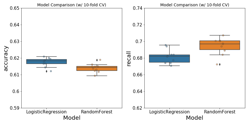
Figure 1. Performance of Logistic Regression and Random Forest classifiers on the training set. Hyper-parameters used in each model were optimezed using grid-search-CV. Left, the accuracy of each model was computed with 10-fold CV. Right, recall score was also obtained with 10-fold cross-validation. Jittered points on box-and-whiskers reflect scores for each of the ten folds.
In general, the two models perform similarly on the test set. Similar AUC scores (~0.69) were obtained by LR and RF (Figure 2).
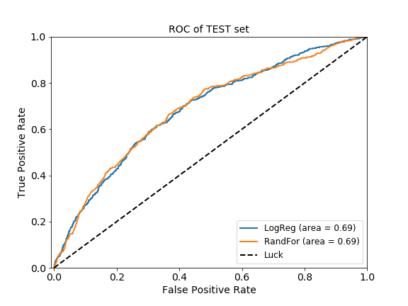
Figure 2. ROC curves of the LR and RF classifiers. Curves were generated with the predicted and the true target values of the test set. Diagonal dashed line indicates random chance.
Higher recall score in the RF classifier means that we are better at detecting obesity in people, which potentially means saving more lives! The RF classifier has fewer False Negative (191) than the LR (229), as illustrated in Figure 3. This means, we would have saved additional 32 people by using the RF classifier instead of LR.
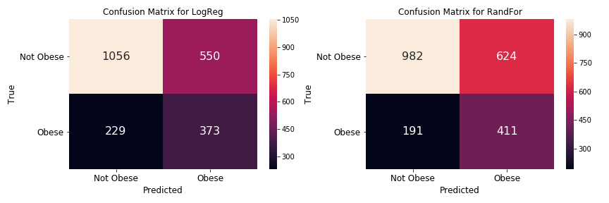
Figure 3. Confusion matrices for LR and RF classifiers. These diagrams were generated using true and predicted target values of the test set.
Recovering Model Interpretability. Although the RF classifier is known to be a robust model with high predictive power, it is a “black-box”-like model due to its low interpretability. To recover some of this aspect, I decided to use Local Interpretable Model-agnostic Explainer (LIME). This package allows us to investigate the effect of feature-variation on the prediction result. For instance, a given individual is predicted to be obese by the RF classifier, with P(obese) of 0.59 (left of Figure 4). We could calculate how the P(obese) changes with the increase of a particular feature, or a combination of features. For this subject, the individual did not participate in any type of exercises, i.e. 0 exerciseFrequency (right). However, if a physician were to suggest an exercise plan for this individual, such as suggesting 4 exercises a week (i.e., increasing exerciseFrequency from 0 to 4), then the P(obese) would decrease to 0.56, indicating that this person would have lower chances of becoming obese. This type of calculation can be performed for each feature, or any combinations of features, at any increments. LIME outputs the overall effect of feature changes on the prediction probabilities (middle of figure).
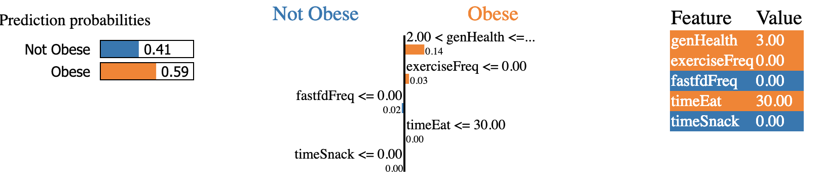
Figure 4. Output of LIME on RF predictions on a given individual. Left, prediction probabilities for a given individual. Middle, the average impact of each feature on the probability of being obese, P(obese). This figure is representative of case_ID #001 (i.e., a single observation in the test set).
In conclusion, using RF and LIME together to predict the chances of obesity seems to be an appropriate approach, as this combination provides both predictive power and interpretability.
Future work
-
Model improvement. Interpretability is an important issue in the healthcare sector, because a physician needs to be able to explain to clients how a particular action/habit may lead to a certain outcome. For this reason, implementing a simple interpretable model like logistic regression would be suitable. So, exploring feature engineering for a logistic model would be one option that I’d like to investigate in the future. In particular, I’d be interested in applying various feature transformations, (especially) because the variables were not normally distributed. I’d like to also see the impact of adding more features to the current model (only 5 were considered at this point). Alternatively, I’d like to explore other combinations of LIME and ensemble models, to get a better predictive power yet maintain some of the explainable aspect.
-
Collect more data. Currently, only 6 years worth of data are available, and the data span from 2006 to 2008 and from 2014 to 2016. I’d like to collect more data (as they become available) and retrain my model. I’d also be interested in looking at non-survey data from elsewhere, because the current project hinges upon the assumption that the experimental data is reliable. In other words, I had assumed that people who were surveyed would answer those questions accurately. In reality, I’d suspect that there would be some inconsistencies, i.e., people are forgetful, or people may feel apprehensive about sharing private information, etc. Furthermore, the current survey questions were focused on individuals’ habits over the past 7 days, which may not be a representative of a person’s “true” lifestyle. For instance, an obese individual who happened to have started a new diet & exercise routine (during the surveyed week) would have answered these questions in a way that reflects his/her “new” lifestyle, as opposed to the previous one. Lastly, I’d like to try using other metrics that describe obesity better. The target response used for this model is based on BMI, which may not be indicative of obesity. For instance, someone who has a great body mass (e.g., a crossfitter or bodybuilder) is typically considered obese, based on BMI. So playing around with this target measure may give a more insightful outcome.
Data sources and tools used
- American Time Use Survey (ATUS) Eating & Health Module Microdata Files
- Data acquisition:
Postgresql,csvkit - Data analysis:
Pandas,seaborn,LIME - Models:
scikit-learn(i.e., Logistic Regression & Random Forest) - Model deployment:
D3,Flask, hosted onHeroku