Was Russell Wilson Underpaid?
Project Goal
- Predicting NFL Player Salary Based on Early Career Perfomance
Introduction
This project was completed during my third week at Metis data science bootcamp. Based on the curriculum, the focus of this project were web-scraping and linear regression models. Unlike the first project, this one was completed individually, i.e., I had the opportunity to determine the scope of the project and to design a way to collect-, clean-, and analyze the data. To this end, I decided to focus my work on NFL analytics.
Having recently moved to Seattle (for the bootcamp), it was the perfect time for me to see the lives of Seattelites through the eyes of their beloved football team, the Seahawks. This team has demonstrated their field-dominance in recent years, as they achieved a Super Bowl victory (in 2013) with their quarterback, Russell Wilson. Wilson’s rise-to-fame story is a perfect example of the moneyball success. As the 75th-pick overall (3rd round), Wilson was drafted by the Seahawks and was signed to a 4-year contract deal that was worth $2.9 million. With less than 1 million annual salary, he took the Seahawks to Super Bowl twice, brought home the Lombardi once, and broke several franchise records. During this period, many (including myself) contended that Russell Wilson deserved higher salary. However, were there any data that support this intuition? In other words, compared to his peers, was Russell Wilson really underpaid during his early NFL career?
In my attempt to answer this question, I wanted to find the value of a player with respect to their early NFL career performance
Project Description and Approach
Each player that is drafted into the NFL typically gets a 4-year contract deal (1st-round players get a 5th year option). Under this contract, a player is unable to renegotiate his salary, even if he excels beyond the franchise’s expectations. Given a set of performance measures, what would be the “market value” ($$$) of a player, e.g., on their 4th year?
Data Acquisition
The scope of my project was limited to 3 types of offensive positions: quarterbacks (QB), running backs (RB), and wide receivers (WR). My approach in assessing players’ early career performance was to collect data that describe their (1) draft worthiness, (2) their first four years of performance stats, (3) and their 4th year salary. These data were webscraped using beautifulsoup and selenium from pro-football-reference and spotrac. The gruesome details of webscraping and preprocessing are described elsewhere, and the codes are available in my repo. Briefly,
-
Draft worthiness - represent players’ physique info and NFL combine results. I chose to use these features, to build upon similar studies by others (ref-1, ref-2). The data include players’ name, draft status, draft round, weight, height, and 40-yard dash record (other results were excluded due to missing values). My analysis was limited to players entering the NFL between 2000 and 2014 (Pro-football-reference.com only has records for rookies that enter the league in year 2000 and later).
-
Four years of performance measures - represent position-specific yards (Yds) and touchdowns (TD) accumulated by each player within the first 4 years of his career. Web-scraping and preparing the datasets were very time-consuming. For a given rookie QB that entered the NFL in 2012, the total passing Yds and TDs for each of the 4 years were scraped from different pages (see Figure 1). Additionally, these stats had to also be collected for each the 3 different positions. Passing, rushing and receiving Yds (or TD) were extracted for QB, RB, and WR, respectively.
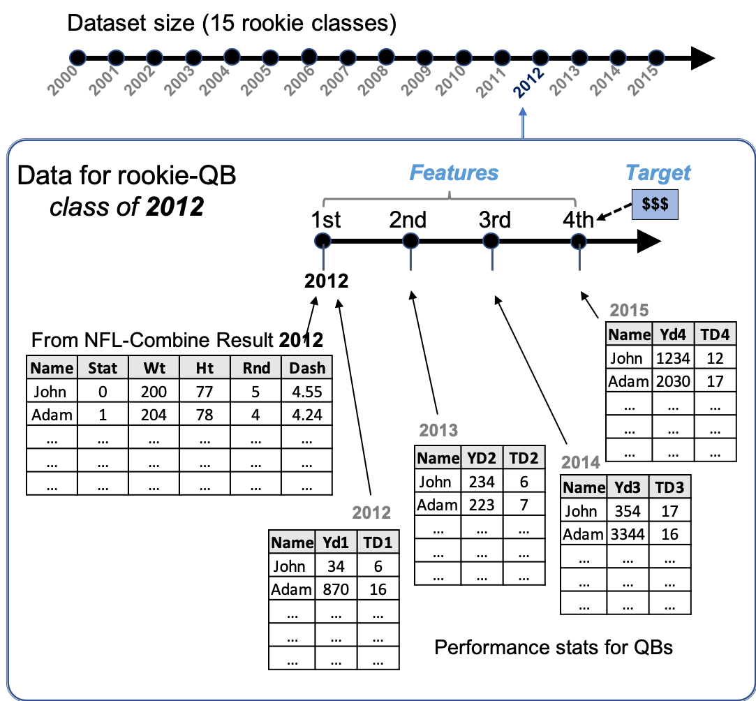
Figure 1. Workflow of data acquisition. Inset illustrates data collection required for a single class of rookie QB entering the NFL in 2012.
-
The 4th year base salary of each player - was used as the target value for my model (see Figure 1). I chose to use this 4th-year information, so that I could target “active” players (i.e., those still playing in NFL at their 4th-year) like Russell Wilson. I collected players’ salaries over the 15-year period of 2003-2015. I also recalculated each year’s salary using the annual inflation rate, to reflect a value that is relevant today, 2018.
Data Wrangling and Feature Engineering
With the workflow described above, I ended up collecting 45 dataframes (i.e., 15 per position), representing 15 years of performance data. However, I couldn’t directly combine all of these dataframes into one table, as the stats correspond to different positions. For instance, the value of rushing Yards may not be identical with passing Yds, nor receiving Yds. So, I decided to normalize the weight of Yds and TDs for each of these different positions using a standard Yahoo fantasy football point system:
- For RB, 1 point for every 10 rushing yards, and 6 points for every TD
- For WR, 1 point for every 10 receiving yards, and 6 points for every TD
- For QB, 1 point for every 10 passing yards, and 4 points for every TD
After transforming players’ Yds & TDs into points, I merged the 45 dataframes together into a single table. Categorical features (such as position and draft status) were one-hot encoded, and one of each of these category-columns was dropped, to avoid the dummy variable trap. Some features were also tranformed using the log1p or box-cox or Yeo-Johnson method. Many of these features were largely skewed to the right, as rookie players often make little impact in their first 4 years of NFL career.
Regression Models and Analysis
After cleaning my dataset and removing “non-active” players (i.e., those who didn’t get paid on their 4th year), I ended up with 356 rows of players and 11 features. (By the way, it was quite remarkable to see that almost 70% of new players entering the NFL didn’t last 4 years). The 11 features I included in my model were draft status, draft round, weight, height, 40-yard dash, 4 years of performance points (i.e., Year1, Year2, Year3, and Year4), and positions (RB or WR) (Figure 2).
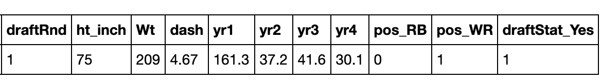
Figure 2. A sample observation from the dataframe containing 11 features. Player names are excluded in the regression models.
Prior to building a regression model, I split the dataframe into training (80%) and testing (20%) sets. With the training set, I built a pipeline that runs feature scaling and 10-fold CV on LinearRegression, Ridge, Lasso, ElasticNet. (Regularization parameters for Ridge, Lasso and ElasticNet were obtained using LassoCV, RidgeCV, and ElasticNetCV). For comparison, I also included tree-based regressors:RandomForestRegressor, DecisionTreeRegressor, andBaggingRegressor, without any hyperparametric tuning.
The result of 10-fold CV on each of the regressors was not as optimal as I had hoped. All linear regression models showed comparable results (Figure 3) with root-mean-squared error (RMSE) of ~0.61, lower than tree-based methods (RMSE~0.64-0.85). Also, r-squared values for linear regressors were abput ~0.21, higher than the those of tree-based regressors, ~0.12.
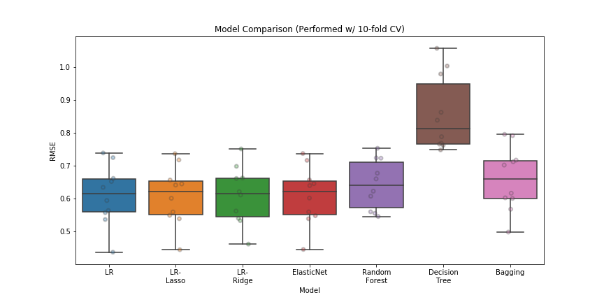
Figure 3. Model-performance on the training set, based on 10-fold CV. Jittered points reflect errors on each fold.
I decided to use the simple linear regression model, without regularizations, to predict players’ salary on the test set. I chose to use the simplest interpretable model, as it be useful for NFL managers in assessing their players.
The linear regression model is fairly effective in predicting players’ salaries (Figure 4). The prediction (orange line) seems to capture the bulk distribution of players’ salary ranging from 0 to ~2 million USD. However, it shows weaker predictive power for high-income players receiving ~4-8 million USD. This model’s tendency to predict lower salary is most likely influenced by the skewed distribution of features (described earlier). Although various transformations were applied, many of those features had outliers at or near zeros (data not shown). Overall, the curent model has an (RMSE) error of ~1 million USD, which is considered substantial for (rookie) players.
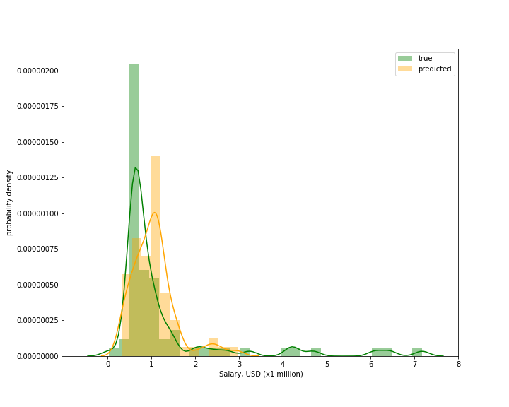
Figure 4. Predicted and true target values in the test set. Predicted- and true salary are illustrated using kernel density estimation, which estimates the probability density function. The horizontal (x-axis) represents salary distribution in the test set, whereas vertical (y-axis) shows the probability density of a given salary.
Once I optimized my linear regressor on the training set, I used it to predict Russell Wilson’s salary, given his performance stats and NFL combine results. The result suggests that an NFL player with his stats should receive ~2.6 million USD, which is higher than Wilson’s actual pay (<1 million/year). Even when the error is considered (~1 million), Wilson’s value should be around 1.6 million USD. So, I would contend that indeed the Seahawks got a very good deal by signing Wilson with a 4-year contract for only ~3 million USD. In other words, given his performance, Russell Wilson could (should) have been paid more that he received.
Summary and Future Work
As it turns out, this classic “moneyball” problem (though successful in MLB) may not be as trivial to achieve in the NFL. At the moment, my model only considers features that are related directly to the individuals, i.e., their performance stats and NFL combine results. However, I believe there are other factors that could affect the value of an NFL player and provide higher predictive power. For example, I would have wanted to include variables that represent a player’s opportunity to play in a game (e.g., playing time per game, number of injured players in the depth chart, etc.).
In addition, I would have wanted to create different regression models for the 3 offensive positions and to use a bigger dataset to train each model. Currently, only one model was used to predict salaries for the 3 types of offensive players, QB, RB, and WR, due to limited number of training datapoints (356 total players). It is important to note that the 4-year-survival rate for NFL players is pretty low, ~30-40%. Not too many players actually last 4 years and longer. Also, pro-football-reference.com only keeps NFL-Combine stats for players entering the NFL from year 2000 and later, which further limits the number of available datapoints. In essence, the challenge of building robust models from limited number of observations remains difficult to accomplish, even in the NFL.
At the end of this NFL analytics project, I felt like I learned so much in building an end-to-end data science pipeline. Through this process, I learned how to web-scrape data from multiple sources, create python scripts to streamline the data preparation process, build simple predictive models, and extract informative insights from them. I can’t wait to work on my next project, so stay tuned for my next installment.
Thanks for reading. A more detailed explanation of my codes is available on my repo. Any helpful comments and suggestions are appreciated.
Attribution
This project was inspired by the work of Ka Hou Sio and Jason SA, who investigated the valuation of NBA and MLB players at METIS.